Bayesian Virtual Site Fitting¶

Virtual sites are useful dummy charge-carrying particles that are not constrained to atomic nuclei, allowing for additional positional flexibility. Here, we implement a Bayesian virtual site fitting algorithm using Pyro with the OpenFF Recharge virtual site formalism.

The full runnable script is at examples/tutorials/bayesian_vsite_fitting.py.

1. Molecule, Conformer, and Multipoles¶

As in the previous examples, we generate a GDMA record for a molecule. In this case, chloromethane.

from openff.recharge.utilities.molecule import extract_conformers
from openff.toolkit import Molecule

from pympfit import GDMASettings, MoleculeGDMARecord, Psi4GDMAGenerator

molecule = Molecule.from_smiles("CCl")
molecule.generate_conformers(n_conformers=1)
[conformer] = extract_conformers(molecule)
settings = GDMASettings()
coords, multipoles = Psi4GDMAGenerator.generate(
    molecule, conformer, settings, minimize=True
)
record = MoleculeGDMARecord.from_molecule(molecule, coords, multipoles, settings)

2. Virtual Site Collection¶

We instantiate a VirtualSiteCollection object with placeholder charge_increments and distance values. These will be sampled during Bayesian inference.

from openff.recharge.charges.vsite import BondChargeSiteParameter, VirtualSiteCollection

vsite_collection = VirtualSiteCollection(parameters=[
    BondChargeSiteParameter(
        smirks="[#17:1]-[#6:2]", name="EP", distance=0.0,
        charge_increments=(0.0, 0.0), sigma=0.0, epsilon=0.0, match="all-permutations",
    )
])

3. Objective Term¶

Next, create an objective term that specifies the vsite position being constrained to somewhere along the C–Cl bond ([#17:1]-[#6:2]). The BondCharge specification places the virtual site along the bond axis.

from pympfit.optimize import MPFITObjective

[objective_term] = list(MPFITObjective.compute_objective_terms(
    multipole_records=[record],
    vsite_collection=vsite_collection,
    _vsite_charge_parameter_keys=[("[#17:1]-[#6:2]", "BondCharge", "EP", 0)],
    _vsite_coordinate_parameter_keys=[("[#17:1]-[#6:2]", "BondCharge", "EP", "distance")],
))

4. Bayesian Model and MCMC Sampling¶

Following standard Pyro recipes, we wrap a forward model function that sets priors for trainable parameters. The model is then passed to the MCMC NUTS algorithm for sampling.

import numpy as np
import pyro
import pyro.distributions as dist
import torch
from pyro.infer import MCMC, NUTS

n_atoms = molecule.n_atoms
targets = [
    torch.from_numpy(r.astype(np.float64).flatten())
    for r in objective_term.reference_values
]


def model():
    # Priors
    free_charges = pyro.sample("free_charges", dist.Normal(
        torch.zeros(n_atoms - 1, 1, dtype=torch.float64), 0.5))
    charge_inc = pyro.sample("charge_inc", dist.Normal(
        torch.zeros(1, 1, dtype=torch.float64), 0.2))
    distance = pyro.sample("distance", dist.Normal(
        torch.tensor([[1.5]], dtype=torch.float64), 0.5))
    sigma = pyro.sample("sigma", dist.HalfCauchy(
        torch.tensor([[0.1]], dtype=torch.float64)))

    preds = objective_term.predict_from_free_charges(free_charges, charge_inc, distance)

    # Likelihood
    for i, (pred, target) in enumerate(zip(preds, targets)):
        pyro.sample(f"obs_{i}", dist.Normal(pred.flatten(), sigma), obs=target)


print("\nRunning NUTS (200 warmup, 500 samples)...")
mcmc = MCMC(NUTS(model), num_samples=500, warmup_steps=200, num_chains=1)
mcmc.run()

Example output (click to expand)

Running NUTS (200 warmup, 500 samples)...
Warmup:   0%|    | 1/700 [00:00,  8.91it/s, step size=2.25e-01, acc. prob=1
...
Sample: 100%|██| 700/700 [00:24, 28.87it/s, step size=4.11e-01, acc. prob=0.933]

Atom charges:
  C1: -0.5736 +/- 0.3150
  Cl2: -0.5850 +/- 0.2218
  H3: +0.3084 +/- 0.3073
  H4: +0.3169 +/- 0.2937
  H5: +0.5332 +/- 0.3753

Vsite charge increment: -0.0041 +/- 0.1894
Vsite distance: 1.512 +/- 0.493 Å

5. Visualization¶

The distribution of the vsite’s charge increment and position along the bond can be visualized using ArviZ trace plots. The trace plot shows both the sampling history (left) and posterior distribution (right).

import arviz as az
import matplotlib.pyplot as plt

idata = az.from_pyro(mcmc, log_likelihood=False)

idata.posterior["vsite_charge_increment"] = idata.posterior["charge_inc"].squeeze()
idata.posterior["vsite_distance_A"] = idata.posterior["distance"].squeeze()

az.plot_trace(idata, var_names=["vsite_charge_increment", "vsite_distance_A"])
plt.tight_layout()
plt.savefig("bayesian_vsite_trace.png", dpi=150)

Bayesian vsite trace plot

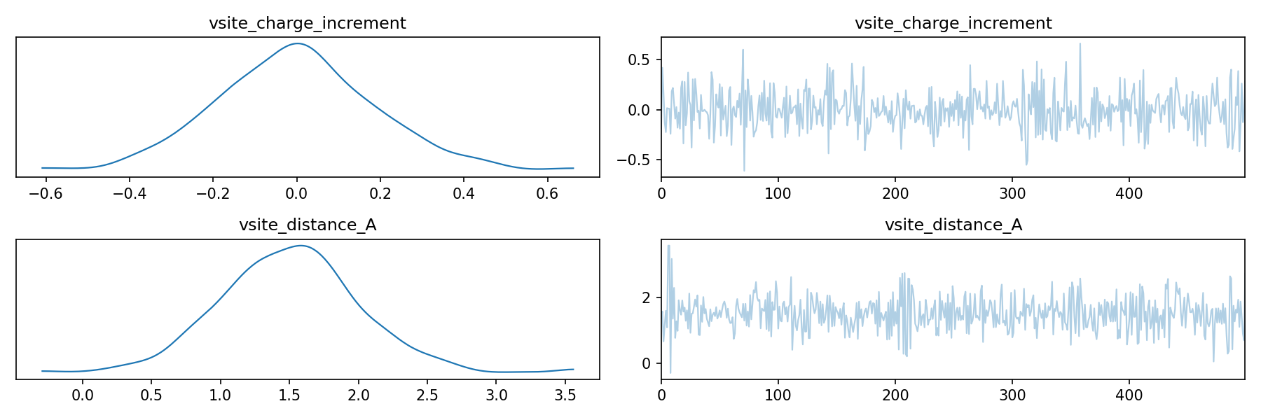
As can be seen, the distribution of the vsite’s charge and position along the bond results in a normally distributed posterior centered near the prior means.